Logistic Function

A logistic function or logistic curve is a common "S" shape (sigmoid curve), with equation:

$$ f(x)=\frac{L}{1+e^{-k\left(x-x_{0}\right)}} $$

e = the natural logarithm base (also known as Euler's number),
x0 = the x-value of the sigmoid's midpoint,
L = the curve's maximum value, and
k = the logistic growth rate or steepness of the curve

Logistic-curve

Adaption to the Interval

$a<y<b, \ 0<x<n$

The idea here is to provide an interval a, b which we would like y to ramp between, over a period x from 0 to n.

Using $L = 1$, and $x_0 = n/2$, we get the sigmoid curve from $\sim 0$ to $\sim 1$. We can multiply this by $(b-a)$ and add $a$ to force it over the interval we desire, from $a$ to $b$. However, $\sim 0 \neq 0$ and $\sim 1 \neq 1$ so we need to normalize the logistic function first.

from sympy import symbols, init_printing, exp, Eq, lambdify
import numpy as np
init_printing()

e = exp(1)
f,g,n,k,x,a,b,o = symbols('f(x),g(x),n,k,x,a,b,o')

L = 1
x0 = n/2
S = lambda x: L/(1+e**(-k*(x-x0)))
S2 = lambda x: L/(1+e**(-k*(x-x0-o)))
norm = lambda y,ymin,ymax: (y-ymin)/(ymax-ymin)

N = norm(S(x),S(0),S(n))
N2 = norm(S2(x),S2(0),S2(n))

display(Eq(f,S(x)))

$f(x) = \frac{1}{1 + e^{- k \left(- \frac{n}{2} + x\right)}}$

display(Eq(g,N*(b-a)+a))

$g(x) = a + \frac{\left(- a + b\right) \left(- \frac{1}{e^{\frac{k n}{2}} + 1} + \frac{1}{1 + e^{- k \left(- \frac{n}{2} + x\right)}}\right)}{- \frac{1}{e^{\frac{k n}{2}} + 1} + \frac{1}{1 + e^{- \frac{k n}{2}}}}$

eqn = (N*(b-a)+a).simplify()
eqn2 = (N2*(b-a)+a).simplify()
display(Eq(g,eqn))

$g(x) = \frac{a \left(- e^{\frac{k n}{2}} + 1\right) \left(e^{\frac{k \left(n - 2 x\right)}{2}} + 1\right) + \left(a - b\right) \left(e^{\frac{k n}{2}} - e^{\frac{k \left(n - 2 x\right)}{2}}\right)}{\left(- e^{\frac{k n}{2}} + 1\right) \left(e^{\frac{k \left(n - 2 x\right)}{2}} + 1\right)}$

free_sym = list(eqn.free_symbols)
free_sym = (np.array(free_sym)[np.argsort([str(x) for x in free_sym])]).tolist()
free_sym2 = list(eqn2.free_symbols)
free_sym2 = (np.array(free_sym2)[np.argsort([str(x) for x in free_sym2])]).tolist()
print('g'+str(tuple(free_sym)).replace(' ',''))

$g(a,b,k,n,x)$

func = lambdify(free_sym,eqn,'numpy')
func2 = lambdify(free_sym2,eqn2,'numpy')

%matplotlib inline
from ipywidgets import interactive
import matplotlib.pyplot as plt
import numpy as np

def _f(a,b,k,n):
    plt.figure(2)
    #n = 20
    #b = 5e-3
    #a = 1e-3
    x = np.linspace(0,n,n)
    y = func(a,b,k,n,x)
    plt.plot(x, y,'.-')
    plt.grid(True,'both','both')
    plt.ylim(bottom=0,top=5)
    plt.ylabel('$\Delta t$ Time Step [ms]')
    plt.xlabel('Iteration Set [1/iterations per step]')
    plt.show()

interactive_plot = interactive(_f, a=(0.,1.), b=(1.1,5), n=(3,25), k=(0.2, 2.),offset=(0,5))
output = interactive_plot.children[-1]
output.layout.height = '300px'
interactive_plot

interactive-plot

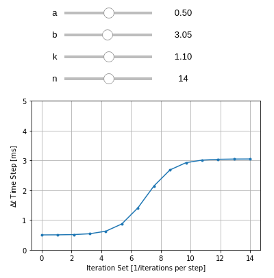
Note: We could move the curve left and right by adding another variable in the equation to alter the term $(x-n/2)$

display(Eq(f,S2(x)))
display(Eq(g,N2*(b-a)+a))
display(Eq(g,eqn2))
print('g'+str(tuple(free_sym2)).replace(' ',''))

$f(x) = \frac{1}{1 + e^{- k \left(- \frac{n}{2} - o + x\right)}}$

$g(x) = a + \frac{\left(- a + b\right) \left(\frac{1}{1 + e^{- k \left(- \frac{n}{2} - o + x\right)}} - \frac{1}{1 + e^{- k \left(- \frac{n}{2} - o\right)}}\right)}{\frac{1}{1 + e^{- k \left(\frac{n}{2} - o\right)}} - \frac{1}{1 + e^{- k \left(- \frac{n}{2} - o\right)}}}$

$g(x) = a + \frac{\left(a - b\right) \left(\frac{1}{e^{k \left(\frac{n}{2} + o - x\right)} + 1} - \frac{1}{e^{k \left(\frac{n}{2} + o\right)} + 1}\right)}{\frac{1}{e^{k \left(\frac{n}{2} + o\right)} + 1} - \frac{1}{1 + e^{- k \left(\frac{n}{2} - o\right)}}}$

$g(a,b,k,n,o,x)$

def _f(a,b,k,n,offset,ylims=[0,5],show=False):
    plt.figure(2)
    #n = 20
    #b = 5e-3
    #a = 1e-3
    x = np.linspace(0,n,n)
    y = func2(a,b,k,n,offset,x)
    plt.plot(x, y,'.-')
    plt.grid(True,'both','both')
    plt.ylim(ylims)
    plt.ylabel('$\Delta t$ Time Step [ms]')
    plt.xlabel('Iteration Set [1/iterations per step]')
    plt.show()
    if show:
        print(x,'\n',y)
        return x,y

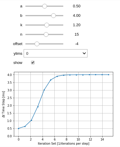
interactive_plot = interactive(_f, a=(0.,1.), b=(1.1,5), n=(3,25), k=(0.2, 2.),offset=(-10,10))
output = interactive_plot.children[-1]
output.layout.height = '500px'
interactive_plot

interactive-plot2

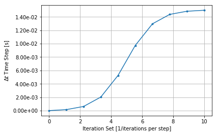
A Static Case

def _f(a,b,k,n,offset):
    plt.figure(2)
    x = np.linspace(0,n,n)
    y = func2(a,b,k,n,offset,x)
    plt.plot(x, y,'.-')
    plt.grid(True,'both','both')
    plt.ylabel('$\Delta t$ Time Step [s]')
    plt.xlabel('Iteration Set [1/iterations per step]')
    import matplotlib.ticker as mtick
    plt.gca().yaxis.set_major_formatter(mtick.FormatStrFormatter('%.2e'))
    plt.show()
    return x,y
x,y = _f(a=1e-7,b=0.015,n=10,k=1.1,offset=0)

png

TUI Commands for Fluent

def command(dt,steps,ips):
    dt = '{0:.4E}'.format(dt)
    string = '''(rpsetvar 'physical-time-step %%dt%%)
(physical-time-steps %%steps%% %%ips%%)
    '''.replace('%%dt%%',str(dt)).replace('%%steps%%',str(steps)).replace('%%ips%%',str(ips))
    return(string)

[print(command(dt,steps=10,ips=50)) for dt in y];

(rpsetvar 'physical-time-step 1.0000E-07)
(physical-time-steps 10 50)

(rpsetvar 'physical-time-step 1.4548E-04)
(physical-time-steps 10 50)

(rpsetvar 'physical-time-step 6.1875E-04)
(physical-time-steps 10 50)

(rpsetvar 'physical-time-step 2.0231E-03)
(physical-time-steps 10 50)

(rpsetvar 'physical-time-step 5.2589E-03)
(physical-time-steps 10 50)

(rpsetvar 'physical-time-step 9.7412E-03)
(physical-time-steps 10 50)

(rpsetvar 'physical-time-step 1.2977E-02)
(physical-time-steps 10 50)

(rpsetvar 'physical-time-step 1.4381E-02)
(physical-time-steps 10 50)

(rpsetvar 'physical-time-step 1.4855E-02)
(physical-time-steps 10 50)

(rpsetvar 'physical-time-step 1.5000E-02)
(physical-time-steps 10 50)

Fluent Temporal Ramp

Logistic Function

Adaption to the Interval

\(a<y<b, \ 0<x<n\)

A Static Case

TUI Commands for Fluent